Scientific Figures Examples for Research and Publication
Explore high-impact scientific figures examples from Nature and Geoscience. Learn to automate publication-quality charts using AI agent workflows.

Communicate complex patterns and evidence by using scientific figures as structured graphical representations. Avoid the common mistake of preserving every raw data point at the expense of the figure’s communicative hierarchy. This practice often results in high-density noise rather than actionable insight.
Use this analysis of specific scientific figures to choose the correct visual framework for data ranging from mobile positioning networks to urban infrastructure cycles. You will learn to balance node density in spatial maps, apply color gradients to represent 24-hour intensity pulses, and use multi-panel layouts to illustrate environmental thresholds. This guide also explains the transition from manual design to agentic workflows using SkillGild’s hosted skills for SVG generation. This approach creates a more efficient process for tracking crisis-driven shifts and synthesizing fine-grained geographic data in 2026.
Key takeaways
- Use multi-panel combination figures to tell a chronological or causal story within a single visual frame.
- Leverage fine-grained mobile and spatial data to create heatmaps that reveal hidden human behavior patterns.
- Automate the generation of SVG-based figures using MCP-compatible agents to ensure resolution independence for print.
- Adopt standardized color palettes and font weights to meet the strict submission guidelines of high-impact journals like Nature.
Try it on a real task: Academic Plotting is free for 25 runs a month.
#Table of contents
- Visualizing high-density mobility and spatial networks
- Mapping temporal shifts in urban infrastructure usage
- Comparing automated figure generation tools for researchers
- Illustrating environmental thresholds through multi-panel layouts
- Tracking crisis-driven travel patterns with comparative heatmaps
- Synthesizing fine-grained time-use data in geography
- Selecting Your Visualization Framework
#Visualizing high-density mobility and spatial networks
Prioritize the hierarchy of spatial nodes to visualize high-density mobility data without creating unreadable "hairball" diagrams. Aggregate raw geographic coordinates into distinct functional clusters or destination hubs when dealing with thousands of individual movement traces. This process reduces the noise of minor deviations and allows the underlying network structure to emerge. Apply thresholding techniques to edge weights to remove low-frequency connections that obscure primary transit corridors. This ensures the reader focuses on the most significant patterns of movement between physical sites.
A successful implementation of this approach is found in a study characterizing destination networks through mobile positioning data, where international tourist movements were mapped across a national scale. This research, published in Tourism Management (Volume 82), demonstrates how to transform millions of discrete data points into a coherent visual narrative. The figure scales node sizes to represent the popularity of specific locations and adjusts edge thickness to indicate the volume of traffic between them. This method allows for the visualization of complex spatial interactions while maintaining geographic context. It provides a clear example of how to manage high-density datasets in a publication-ready format.
Balance node density by choosing between geographic accuracy and topological clarity. Spatial network visualization often employs force-directed layouts constrained by geographic boundaries to prevent overlapping nodes in densely populated urban centers. If nodes are too close, the resulting figure becomes illegible. However, moving them too far from their actual coordinates risks misinforming the reader about the physical distance between destinations. Effective scientific figures examples often resolve this by using inset maps for high-density areas or by grouping minor nodes into larger administrative regions. This preserves the overall flow without sacrificing local detail.
Focus final rendering choices on the contrast between the background geography and the network overlay. Use a muted, desaturated base map to allow the vibrant colors of the mobility network to stand out. Select a color palette that is perceptually uniform. This ensures that the gradient representing movement intensity is interpretable even when printed in grayscale. By combining these structural and aesthetic choices, you convert complex geospatial data into an actionable tool for urban planners and policy makers. This moves beyond raw data points to reveal the functional connectivity of a region.
#Mapping temporal shifts in urban infrastructure usage
Use topographical activity diagrams to visualize how urban systems fluctuate. These figures transform raw GPS or transaction logs into a three-dimensional representation of activity over time. For instance, the paper unraveling the topographical activity and pulses of cycling activities in Computers, Environment and Urban Systems (volume 75) demonstrates this by mapping dockless bike-sharing patterns. This method allows observers to see where bikes are located and the rhythmic "heartbeat" of the city, showing how demand ebbs and flows across different districts.
Apply color gradients to denote intensity across a 24-hour cycle. By using a sequential or diverging color scale, the figure maps the density of usage at specific timestamps. High-intensity periods, such as morning commutes or evening social peaks, are rendered in saturated or warmer tones. Dormant periods appear in cooler, desaturated hues. This gradient approach enables a viewer to distinguish between a static infrastructure map and a dynamic temporal model, highlighting specific hours where system capacity is most strained.
Extend these visuals beyond transit to broader urban geography. A study on tourism geography through time use published in the Annals of the American Association of Geographers (volume 111, issue 5) processes fine-grained mobile phone data to track these shifts. Researchers looking to build similar interactive or high-fidelity visualizations can find technical guidance through the Claude Frontend Design Skill: Setup & Usage course. Mastering these tools ensures that the resulting figures maintain clarity even when representing millions of data points across a temporal axis.
When preparing these figures publication standards, prioritize the legibility of the temporal axis. Ensure the 24-hour cycle is clearly labeled and that the color bar includes specific units of intensity, such as trips per hour or active devices. Avoid overlapping too many data layers, which can obscure the "pulse" effect. By isolating the temporal variable against a simplified spatial background, the figure communicates the specific timing of urban infrastructure usage without overwhelming the reader with extraneous geographic detail.
#Comparing automated figure generation tools for researchers
Transition from manual layout software to agentic workflows to eliminate the repetitive labor of figure updates. Traditional vector editors require researchers to manually adjust every node, line, and label whenever underlying data or peer review feedback changes. This creates a "rebuilding tax" that consumes hours of high-value research time. Modern workflows instead use LLM agents that interpret data schemas and design requirements to generate editable code directly, ensuring that the figure remains a derivative of the source data rather than an isolated, static asset.
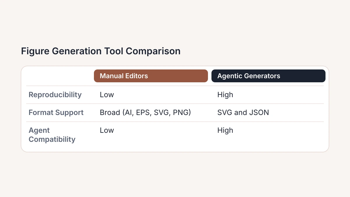
Implement SkillGild’s hosted skills to bridge the gap between raw data and publication-ready SVG files. These specialized tools allow agents to execute precise visualization logic, handling complex coordinate mapping and aesthetic styling without manual intervention. Researchers seeking to optimize their workflow can employ the Best Claude Skills for Design & Frontend to automate the generation of diagrams and charts. By offloading the rendering logic to hosted skills, machine learning researchers ensure that figures are consistent across different sections of a paper and easily adjustable via text prompts rather than mouse clicks.
Prioritize tools that support SVG (Scalable Vector Graphics) to maintain visual fidelity during the 2026 publication cycle. Agentic generation reduces the friction of research by allowing for the rapid iteration of loss curves, architecture diagrams, and heatmaps. This approach ensures that when a model is retrained or a dataset is updated, the associated figures can be regenerated programmatically. This shift from "drawing" to "defining" figures allows research teams to maintain high-quality documentation without the overhead of dedicated graphic design cycles.
| Tool Category | Reproducibility | Format Support | Agent Compatibility |
|---|---|---|---|
| Manual Vector Editors | Low; requires manual version tracking | Broad; AI, EPS, SVG, PNG | Low; requires GUI interaction |
| Script-based Plotting | High; via version-controlled code | Broad; PDF, SVG, PNG, JPG | Moderate; requires code execution |
| Agentic SVG Generators | High; via prompt and data state | Primary focus on SVG and JSON | High; native API-driven design |
#Illustrating environmental thresholds through multi-panel layouts
Capture the exact point where one limiting factor supersedes another to visualize how ecosystems respond to environmental stressors. Pinpoint these thresholds with precision by using multi-panel layouts. Standardize the x-axis across several subplots to illustrate how diverse biological or chemical variables react simultaneously to a single driver, such as rainfall or temperature. This approach maintains a direct visual comparison between different ecosystem components without the clutter of over-plotting multiple lines on a single set of axes.
The 'Nature Geoscience' style provides a premier scientific figures example in the paper titled "Precipitation threshold-driven shifts in dominant controls of ecosystem nitrogen retention." This specific layout employs small multiples to demonstrate how nitrogen processes change once a specific precipitation level is reached. Align the figures vertically to show that while several variables may remain stable in arid conditions, they deviate sharply and in unison once the threshold is crossed. This layout succeeds because it treats the threshold as a vertical alignment across the entire figure stack rather than a single data point, making the shift in dominant controls immediately apparent.
Fix the horizontal scale for every panel in the set to execute this style effectively. Each panel should represent a different dependent variable, such as microbial activity, soil moisture, or vegetation cover, on the vertical axis. Keep the x-axis consistent so that any shift in the slope or variance across all panels at the same coordinate indicates a systemic transition. Use a shaded vertical bar or a dashed line to mark the threshold across all panels. This ensures the reader can track the ecological tipping point without moving between disparate charts. Identify lag times or immediate responses across different trophic levels through this consistency.
Minimize redundant labels to maintain clarity when managing the visual hierarchy in these multi-panel figures. Remove the x-axis titles and tick labels from the upper panels, leaving them only on the bottom-most row to reduce the ink-to-data ratio. Reinforce the comparative nature of the data by using consistent color schemes to represent different treatments or sites across all panels. Tag each panel with a bold letter in the top-left corner when preparing these for publication to facilitate clear referencing in the text. Allow the viewer to process complex, multi-variable ecosystem shifts as a single, coherent narrative through this structure.
#Tracking crisis-driven travel patterns with comparative heatmaps
Prioritize delta-change maps over raw volume displays when visualizing sudden shifts in human behavior. Raw data often hides the significance of a disruption by focusing on absolute totals, which may stay high even during a sharp decline. Map the difference between current activity and a historical baseline to highlight the impact of the crisis itself. This approach transforms a standard geographical heatmap into a diagnostic tool that identifies exactly where and how much a system has diverged from its expected state.
A primary example of this technique appears in the Nature Communications study on travel patterns during the early COVID-19 pandemic, which documented shifts in China (Volume 11, Issue 1, pp. 1-9). Rather than simply showing the number of travelers across provinces, the researchers visualized the percentage change compared to the same period in previous years. This method allowed for a direct comparison of the pandemic’s restrictive effects across different urban centers, regardless of their initial population sizes or typical traffic volumes.
The visual effectiveness of these heatmaps relies on a diverging color scale. In the Nature Communications example, the use of contrasting hues to represent positive and negative deviations ensures that the viewer can immediately distinguish between areas of growth and areas of contraction. By centering the scale at zero, which represents no change from the norm, the figure eliminates the need for the reader to perform mental arithmetic. This design choice is particularly useful for publication, as it allows the data to communicate the severity of a crisis across multiple geographic regions simultaneously.
To implement this in current 2026 research, professionals should establish a statistically representative baseline from pre-crisis data before calculating the variance. This technique is not limited to epidemiology; it is equally effective for illustrating market volatility, environmental anomalies, or sudden infrastructure failures. By focusing on the delta, the researcher provides a clearer narrative of disruption than a standard density map could offer. When preparing these figures, ensure the legend explicitly defines the baseline period to maintain transparency and reproducibility.
#Synthesizing fine-grained time-use data in geography
Implement a computational framework for tourism geography to process massive datasets that track human movement with high precision. This methodology is exemplified in the paper Tourism geography through the lens of time use, published in Annals of the American Association of Geographers, volume 111, issue 5, pages 1420-1444. Shift your focus to time-use patterns to move beyond simple arrival counts and understand the duration and sequence of activities within a destination. This framework provides a structure to transform raw signal data into actionable insights regarding visitor behavior.
Processing fine-grained mobile phone data creates a significant visualization challenge because of information overload. Raw datasets often contain millions of individual GPS pings or signal handovers. Plotting these directly onto a map results in illegible "spaghetti plots" that obscure meaningful trends. To maintain clarity, aggregate these points into cohesive temporal and spatial units without sacrificing the granularity that makes the data valuable. Design scientific figures that balance the macro-level trends of a broad population with the micro-level behaviors of specific visitor cohorts.
Adopt a hierarchical figure structure to prevent cognitive fatigue when presenting these complex datasets. Use a multi-panel layout where the primary panel establishes the broad geographic context, while subsequent panels zoom into specific time-use clusters or demographic segments. By nesting detailed data within a broader framework, the figure guides the viewer from the general phenomenon to the specific computational results. This ensures that the high resolution of the mobile data supports the research narrative rather than distracting from the core findings.
When designing figures publications, prioritize visual hierarchy by employing color-coded timelines and density heatmaps. Instead of attempting to display every individual data point, use representative subsets or averaged trajectories to illustrate the results of the computational framework. Ensure that the scale, color ramps, and legends remain consistent across all sub-panels to allow for immediate cross-comparison of different time-use profiles. This systematic approach transforms raw computational output into a persuasive tool for geographic analysis and regional policy planning.
#Selecting Your Visualization Framework
- Identify data dimensionality: determine if your high-density mobility or spatial network requires multi-panel layouts or simplified single-axis representations to remain legible for peer-reviewed publication.
- Verify temporal resolution: assess whether your tracked infrastructure usage shifts necessitate static comparative heatmaps or dynamic time-series animations to convey the specific rate of change to your readers.
- Evaluate automation requirements: select between bespoke Python-based plotting scripts and standardized automated generation tools based on the total size of your dataset and your required update frequency.
- Define critical thresholds: establish if the figure must explicitly highlight specific environmental limits or if it should prioritize showing general trends across the entire data range for broader context.
- Audit visual hierarchy: ensure your synthesis of fine-grained time-use data maintains a clear focal point that guides the viewer toward your primary research conclusion without unnecessary clutter.
Effective scientific communication relies on selecting the right format for your specific dataset rather than simply using the most complex tool currently available. Skillgild offers specialized technical tracks to help you master these advanced visualization techniques for modern research. Start your training today at https://skillgild.dev/.